A linear-time heuristic for improving network partitions
A circuit partitioning algorithm

A linear-time heuristic for improving network partitions C. M. Fiduccia and R. M. Mattheyses DAC'1988
This paper describes the Fiduccia–Mattheyses algorithm which is similar to the Kernighan–Lin algorithm for graph partitioning. The ideas are old, but still very relevant.
Network Partitioning
The object which this algorithm operates on is a network. A network is similar to a graph; the key difference is that edges are replaced with nets. A net connects 2 or more vertices (an edge is a degenerate case which always connects 2 vertices). This makes sense in hardware applications, where vertices are circuit components, and nets are the wires that connect them.
The problem is to divide the vertices in a network into two sets, A and B. Nets which cross from A to B are called cut nets. The number of cut nets should be minimized. The relative sizes of A and B must adhere to a balance criterion which ensures that A and B have roughly the same number of vertices.
The graph partitioning problem is similar to the min-cut problem. The key difference is that in graph partitioning, there is a requirement that the two partitions are balanced (have roughly equal sizes).
Graph partitioning is NP-hard; the algorithm described in this paper is not guaranteed to produce an optimal result.
The Algorithm
The algorithm starts by dividing the vertices into initial sets A and B, ensuring that the balance criterion is honored. It then iteratively executes passes, until no more improvement can be made.
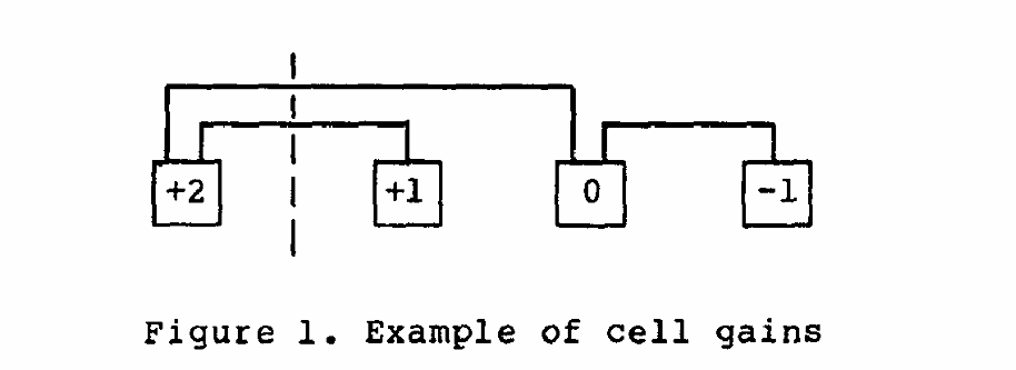
A single pass can potentially move each vertex in the graph (to the complementary partition). Each vertex will only be moved at most once per pass. Within a pass, vertices are sorted according to their associated gain. The gain of a vertex is the overall improvement that would result by moving that vertex to the complementary partition. Fig. 1 has an example. The current partition is represented by the vertical dashed line. The partitioning would be improved by moving the vertex with +1 gain to the left partition (one fewer net would be cut). Partitioning would also be improved by moving the +2 vertex over to the right partition, but the balance criterion would likely not allow this. The partitioning would be made worse if the vertex with -1 gain were to be moved (as the associated net would become cut).
A single pass produces a set of candidate partitions and then chooses the best candidate to be the input partition for the next pass. The algorithm to execute a single pass is:
Among all vertices which have not been considered in the current pass, and which can be moved without violating the balance criterion, select a vertex with maximal gain
Move that vertex and note the updated partition as a candidate partition
After a single pass has completed, examine all candidate partitions the pass produced. Choose the best one. There are two subtle points about this process:
The gain of each vertex is recomputed after each move.
Step #1 will select vertices with negative gains. The idea is that within a pass, a small bad move can unlock future (but within the same pass) good moves. The best candidate partition is selected at the end of each pass, so partitions that directly result from bad moves will be ignored.
Critical Nets
A net is called critical if it is connected to zero or one vertices in A or B. If a net is not critical, then it can be ignored when considering moving a single vertex, because an individual move cannot cause non-critical nets to change from cut to uncut (or the other way around). The gain of an individual vertex can be computed by summing the contributions from all critical nets that vertex is connected to. Each critical net contributes -1, 0, or +1 to the gain of a vertex.
Updating Gains
The following steps enable incremental updates of data structures containing the following information when moving a vertex v from set A to set B:
The gain of each vertex
The number of vertices in A that each net is connected to
The number of vertices in B that each net is connected to
For each net 'n' connected to v:
  if n is not connected to B:
    increment the gain of all other vertices connected to n
  if n is connected to exactly 1 vertex in B:
    decrement the gain associated with that vertex

  decrement the number of vertices that n is connected to in A
  increment the number of vertices that n is connected to in B

  if n is connected to 0 vertices in A:
    decrement the gain of all other vertices connected to n
  if n is connected to exactly 1 vertex in A:
    then increment the gain of that vertex
Note that the conditionals which examine the number of vertices that a net is connected to in A or B only consider critical nets (nets connected to 0 or 1 vertices in the relevant partition).
Selecting a Maximum-Gain Vertex
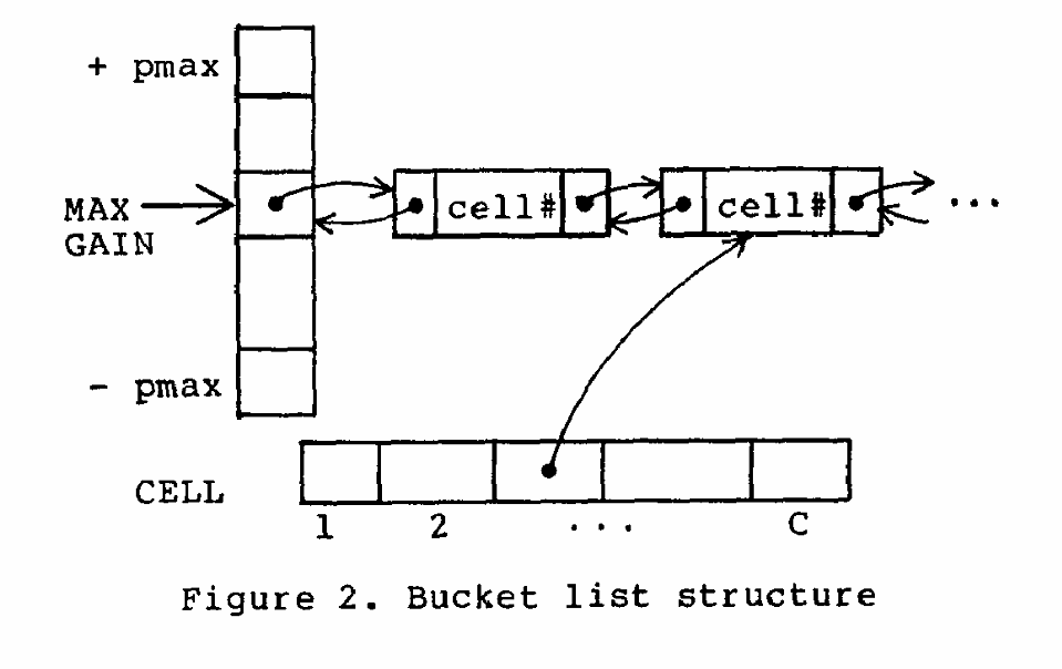
The inner loop of the pass algorithm chooses a vertex with maximum gain. The algorithm above shows how to update the gain associated with each vertex as the pass progresses but does not deal with efficiently selecting a high gain vertex. The trick here is that there is a bounded range of values that a gain can have. The paper calls the bounds [-pmax, pmax]. pmax is simply the maximum degree of any vertex. With this knowledge, vertices can be stored in an array of linked lists. Each entry in the array corresponds to a particular gain value. When the gain of a vertex changes, it can be removed from the list that it is currently contained in and inserted in the list corresponding to the new gain. Fig. 2 illustrates the data structure:
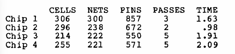
Results
The following table shows performance results for four randomly sampled chips. The average chip has 267 vertices, 245 nets, and the average degree of a vertex is 2650. I would have thought that more passes were needed to converge on a solution.