Pipeline Parallel Decompression

Bribing God

This isn’t a paper summary, but rather a description of a hobby experiment I’ve been hacking on ("research quality" code).

The Potential of Pipeline Parallelism

This quote (attributed to either Anonymous or David Clark) originally referred to networking, but applies to parallel programming as well:

There is an old network saying: Bandwidth problems can be cured with money. Latency problems are harder because the speed of light is fixed—you can’t bribe God.

Standard "cured with money" parallelization techniques (e.g., shared-nothing architectures, data parallelism) try to minimize cross-core communication. These hammers are great for hitting nails labeled: "improve throughput by throwing more cores at the problem”.

Not everything is a nail. Important problems which cannot be solved with this kind of approach include:

• Parallel network packet processing in cases where load balancing schemes like RSS do not apply

• Parallel transaction processing when there is high contention between transactions

• Parallel encryption of a single stream of data

Pipeline parallelism has the potential to provide "bribing God” solutions to some of these problems.

A potential additional benefit that pipeline parallelism brings to the table is better usage of CPU caches because of a smaller working set. For example, if 8 cores cooperate to process 1 input file, the working set (input data, output data, intermediate data structures) is potentially 8 times smaller than the case where each core processes a separate input file. This caching advantage also applies to instruction caches, as pipeline parallelism distributes the computational steps of an algorithm across cores.

Pipeline parallelism has some major drawbacks:

• Fine-grain synchronization/communication

• Load imbalance

The purpose of this experiment is to put some numbers on the costs and benefits in a real-world application (DEFLATE decompression).

Pipeline Design

DEFLATE decompression is hard to parallelize because of two tight feedback loops:

1. The position of encoded token N in the input stream is not known until token N-1 is decoded (because input data is encoded with a variable length code).

2. The output generated by a match (i.e., length & distance tuple) cannot be computed until some amount of previous output has been generated (because a match references previously generated output)

A Negative Nancy might view these as problems, but a Positive Pipeliner views them as a guide for how to decompose the algorithm into pipeline stages. The general technique is to dedicate a pipeline stage to each of these feedback loops and whittle them down to be as tight as possible.

The design I’ve landed on has three pipeline stages: chase, lookup, and output.

The chase stage computes the length of each encoded token. It simply reads the next 13 bits from the input stream and uses them as an index into a lookup table. The inner loop looks like this:

const size_t lut_key_bits = 13;
const uint32_t lut_key_mask = (1 << lut_key_width) - 1;

const uint32_t input_bits = bits.extract<uint32_t>(lut_key_bits);
const uint8_t length = length_lut[input_bits & lut_key_mask];
bits.consume(length);

Note that in contrast to non-pipelined implementations, the only thing this code (and the lookup table) are concerned with is finding the length of each token, everything else is dealt with in another pipeline stage. Each iteration of this loop runs in about 8 clock cycles, and the lookup table fits in the L1 cache. The CPU cannot run multiple iterations of this loop in parallel due to the tight dependency chain.

The input to the lookup stage is the encoded bits associated with each input token (input_bits in the code above). These bits are used to perform another lookup (in a larger lookup table, stored in the L2 cache) which results in much more information about each token. Optimizing this stage is easy, because it doesn’t contain any tight feedback loops. The CPU can process multiple loop iterations in parallel, which enables it to hide the latency of accessing the L2. If necessary, it would be easy to split this pipeline stage into two. The inner loop looks like this:

const output_lookup_result olr = lookup_lut[input_bits & lut_key_mask];

const size_t match_length = olr.match_length;

const uint16_t dist_extra_bits_mask = (1ull << olr.num_dist_extra_bits) - 1;
const uint16_t dist_extra_bits = (cp.input_bits >> olr.offset_to_dist_extra_bits) & dist_extra_bits_mask;
const size_t match_dist = olr.base_dist + dist_extra_bits;

The olr structure contains metadata about the input token (literal value and/or information about a match). This data structure does not contain the exact distance associated with the match, the variables named extra_bits deal with that detail from the DEFLATE spec.

The output stage writes literals and matches to the output buffer. This code leans on the CPU store-to-load forwarding hardware to deal with match operations which must read data that was recently produced. Each iteration of the inner loop performs a word-sized write of literal data, plus a 32B read and write to read and write match data. Actual store-to-load forwarding is rare, as most match distances are large.

*curr_result_ptr = literals;
curr_result_ptr += literal_count;

const uint8_t* src = curr_result_ptr - match_dist;
uint8_t* const dst = curr_result_ptr;

const __m256i src_data0 = _mm256_loadu_si256(reinterpret_cast<const __m256i*>(src));
_mm256_storeu_si256(reinterpret_cast<__m256i*>(dst), src_data0);

Results

The Silesia Corpus contains commonly used files to benchmark compression algorithms. dickens has English text with short matches whereas nci contains data dumps with longer matches.

libdeflate is an optimized library which can decompress roughly 2-3x faster than the standard zlib.

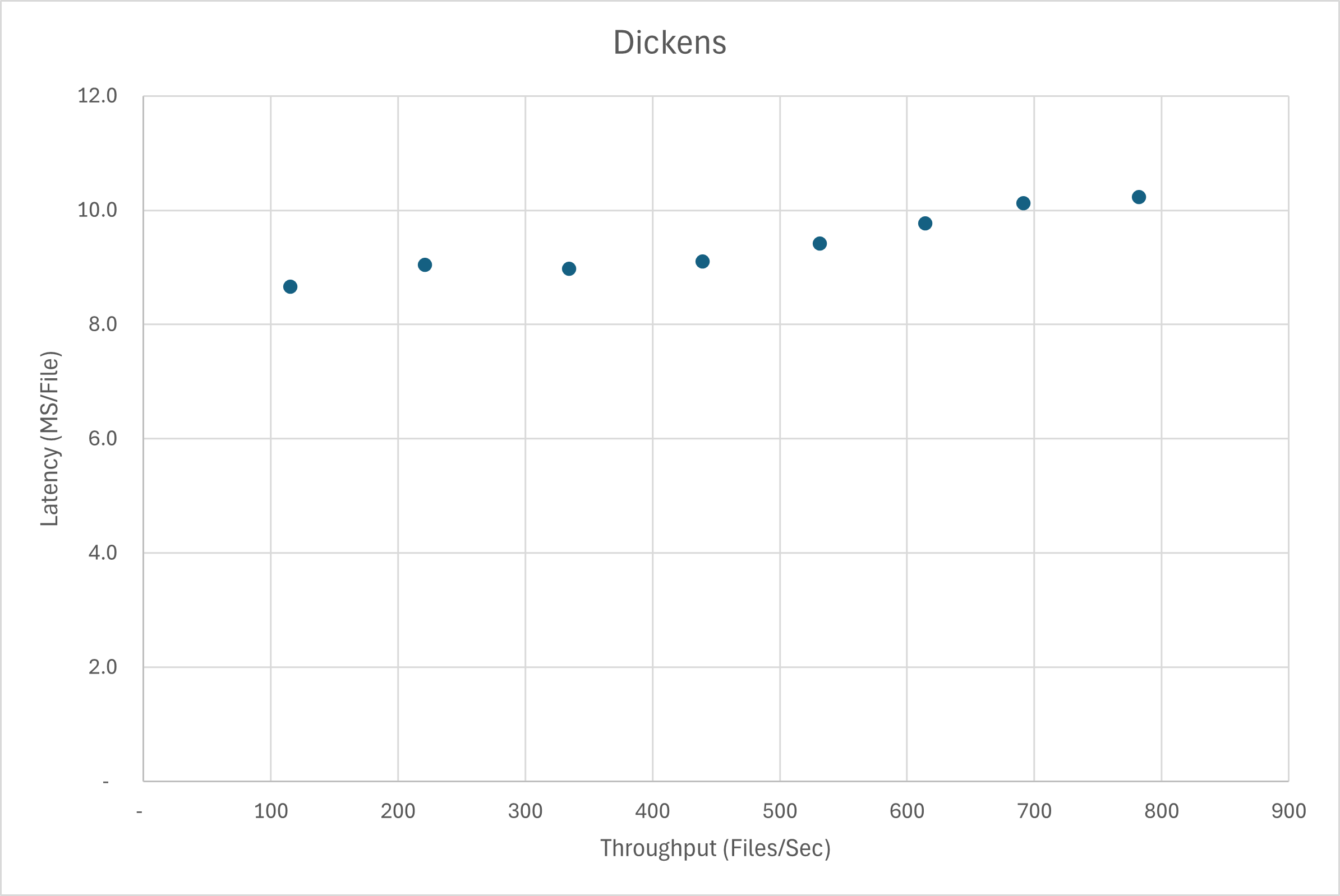
The following chart shows baseline libdeflate performance on dickens in a shared-nothing architecture where each CPU core decompresses a separate input file. There is one data point for each core count (1, 2, …, 8). As you would expect, throwing more cores at the problem improves throughput, at the cost of slight latency increase. If you want a more interesting tradeoff of throughput vs. latency, you have to bribe God. For example, say you are writing a decompression application. If the user requests a bulk decompression of 100 files, then the optimal choice may assign each file to a CPU core. But if the user requests to decompress a single file, then you would prefer to decompress using multiple CPU cores.

And here is the same chart with the 3-stage pipeline implementation added in orange (compare it to the third blue dot from the left for a 3-core vs 3-core comparison):

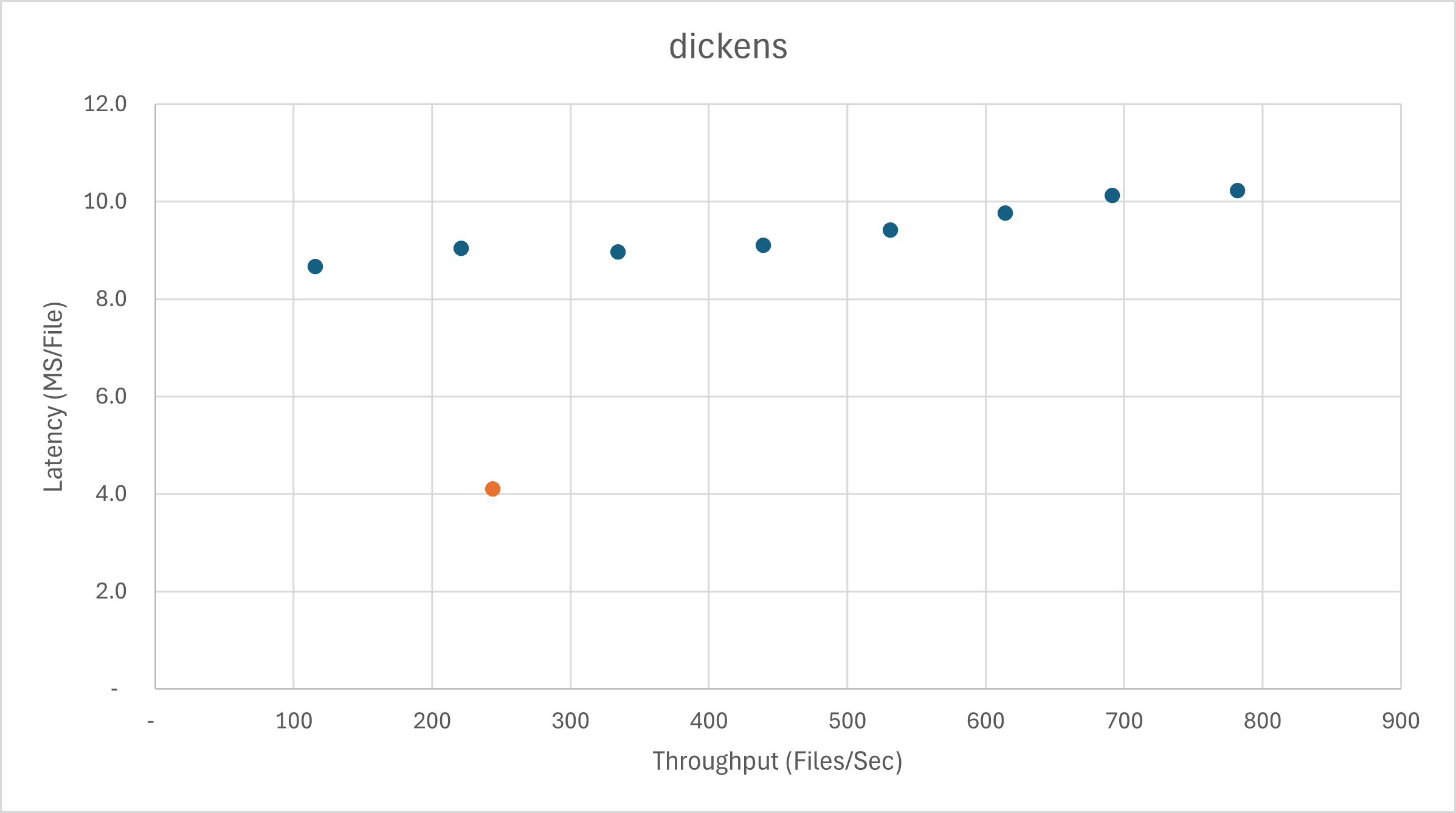
For a 37% cost in throughput, you get a 2x reduction in latency.

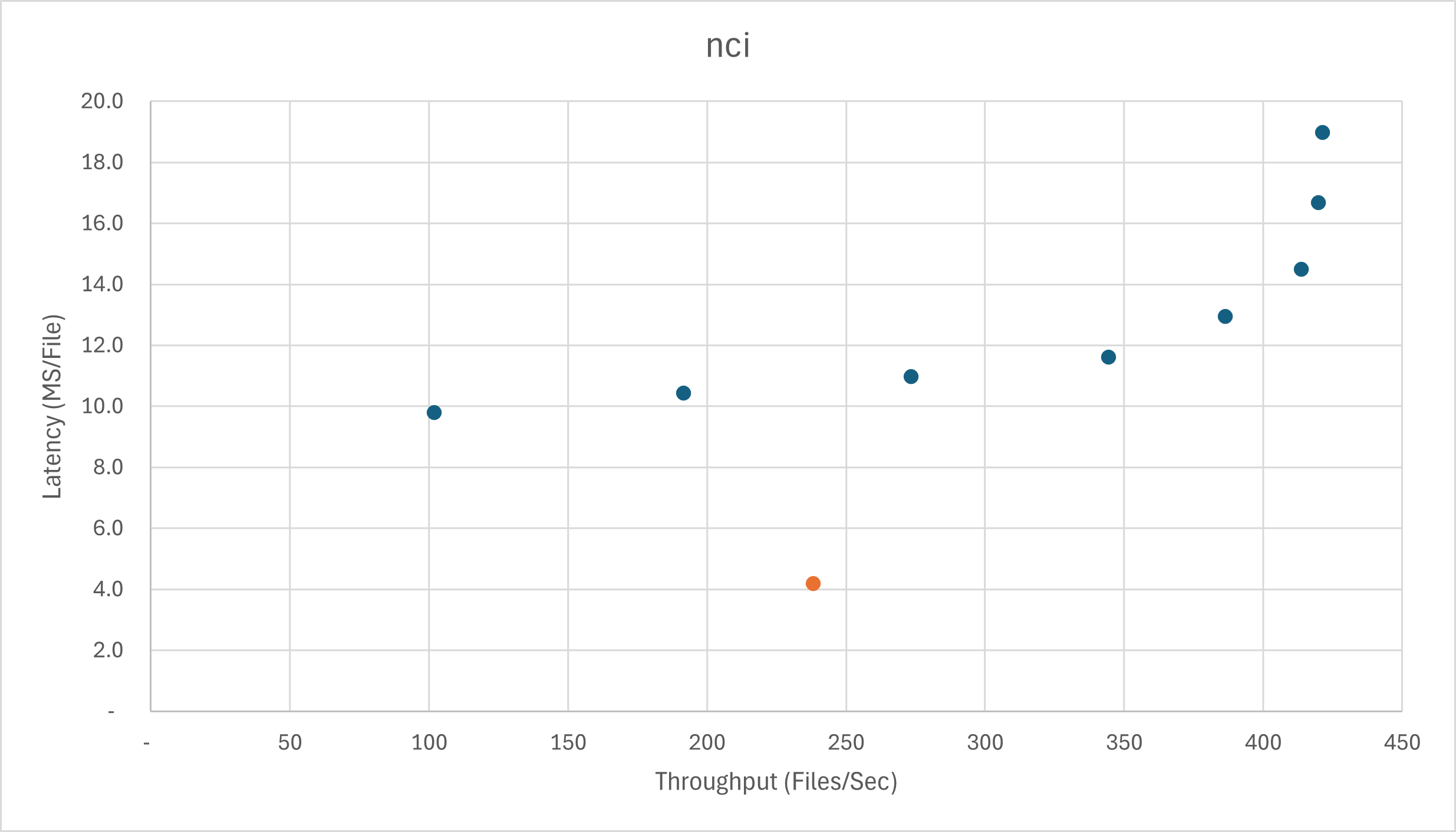
Here is the chart for nci, which shows a similar story. Data-parallel throughput saturates at 6 cores. Pipeline parallelism allows a 2.6x latency reduction at the cost of 14% throughput.

Dangling Pointers

I think there is room for language/runtime support to improve performance of pipeline parallel algorithms on multicore CPUs (by reducing load imbalance).

dickens is bound by the chase stage, whereas nci is bound by the output stage. The programmer could supply multiple implementations of the pipeline (with some compiler help to reduce code duplication), and the runtime could dynamically switch between them depending on which stage is the bottleneck.

High level synthesis tools are capable of automatic pipelining. Such techniques could be used to automatically generate many pipeline implementations for the runtime to choose between.

Tricks

The description above leaves out a few implementation details regarding the lookup tables. Because the lookup table data is spread across two cores (i.e., pipeline stages), there is enough room to store data for 2 Huffman tokens (2 literals, or a full match). This provides a large speedup compared to traditional implementations that store all data in the caches of a single core.

Because the lookup stage is throughput bound rather than latency bound, it can afford to access the lookup table via a layer of indirection. The 13 input bits are used to lookup a uint16_t index, and that index is used to access the final data in another lookup table. The second lookup table has fewer entries, but each entry is larger. This reduces the total working set.

Branch Prediction

This design leans heavily on CPU branch prediction. The code snippets shown earlier are for the common cases, with branches used to implement uncommon cases (e.g., a single encoded token that is wider than 13 bits). As long as those cases are rare, branch prediction does a great job of keeping the inner loops humming.

Ghost in the machine

An interesting puzzle arose during this experiment. I found that performance could swing widely (~10%) based on where the operating system located stacks of the various threads. The stack address would change from run to run because of ASLR. A little alloca to offset the stack by a small amount would resolve this issue. It seems to be an important consideration when trying to maximize usage of the L1 cache.