Accelerate Distributed Joins with Predicate Transfer

Reducing shuffle traffic in distributed joins

Accelerate Distributed Joins with Predicate Transfer Yifei Yang and Xiangyao Yu SIGMOD'25

Thanks to

Yifei Yang

for “dereferencing” this dangling pointer from the prior post on predicate transfer. This paper extends prior work on predicate transfer to apply to distributed joins.

Predicate Transfer Refresh

If you have time, check out my post on predicate transfer. If not, an executive can derive a summary from Fig. 1:

Source: https://dl.acm.org/doi/10.1145/3725259

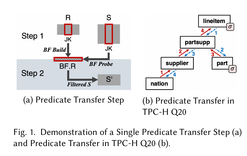
The idea is to pre-filter the tables involved in a query, so as to reduce total query time by joining smaller tables. Fig. 1(a) shows two tables which will be joined during query execution: R and S. S' is the pre-filtered version of S. S' is constructed with the following steps:

1. Iterate through all join keys in R, inserting each key into a bloom filter (BF.R)

2. Iterate through all rows in S, probing BF.R for each row, insert rows that pass the bloom filter into S'

Now that S' is constructed, the algorithm takes another step in the join graph (illustrated in Fig. 1(b)). In this next step, the S' computed in a previous iteration performs the job of R (a different join key is used in this step). The algorithm starts at tables with pushed-down filters, propagates predicate information forward through the join graph, and then reverses and propagates predicate information backward.

Now that you remember the basics of predicate transfer, it’s time to deal with distributed joins. In such an environment, each node in the system holds a subset of each table (e.g., R and S).

Broadcast

If R is small relative to S, then it makes sense to broadcast BF.R to each node. Fig. 3 illustrates three ways to do this:

Source: https://dl.acm.org/doi/10.1145/3725259

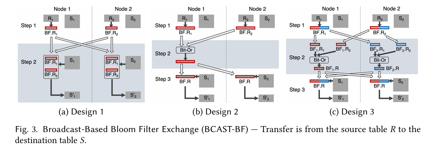
(a) Design 1 is the simplest, let’s start there. It is a two-step process to compute the pre-filtered version of S (i.e., S').

1. Node i iterates through all rows in its local subset of R, and inserts each join key into a local bloom filter BF.Ri. Each of these small bloom filters is broadcast to every other node (which isn’t too expensive because R is assumed to be small).

2. Node i iterates through all rows in its local subset of S, and probes all of the small bloom filters (BF.R1, BF.R2, …). If any probe operation results in a hit, then the row is inserted into the local subset of S'.

Design 2 merges all of the small bloom filters together to avoid multiple probes, and design 3 parallelizes the merging process.

Shuffle

If both tables are roughly the same size, then shuffling is likely more efficient. Shuffling is based on the following property of relational algebra (this is the 3rd post with this same formula):

\((R \Join S) = (R_{h_0} \Join S_{h_0}) \cup (R_{h_1} \Join S_{h_1})\)

In English: partition R and S into two partitions (based on hashing the join key) and then perform partition-wise joins.

In the distributed setting, the number of partitions can equal the number of nodes.

Fig. 4(b) illustrates shuffle-based predicate transfer with (N=2) nodes:

Source: https://dl.acm.org/doi/10.1145/3725259

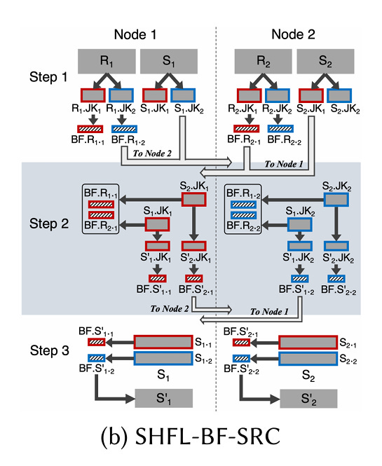
1. Node i partitions its local subset of R and S into N partitions (Ri.JK1, Ri.JK2, …), using a hash of the join key to assign each row to a partition. Partitions of R are only used to compute local bloom filters (one per partition). The resulting bloom filters and partitions of S are sent across the network. For example, Si.JK2 is sent to node 2, and similarly the bloom filter derived from Ri.JK2 is sent to node 2.

2. Each node iterates through all join keys in the partition of S that it just received, probing all bloom filters. If there is a hit in any bloom filter, then the join key is inserted into one of N bloom filters (the bloom filter index depends on which node the row originally came from). These bloom filters are sent back to the associated nodes.

3. Each node iterates through its local subset of S. For each row, the join key is used to determine which node computed the corresponding bloom filter. That bloom filter is used to check to see if the row should be inserted into the local subset of S'.

In step 2, each node acts like an RPC server: it handles requests and sends responses. The request payload is a subset of S. The response payload is a bloom filter which represents the subset of that subset which should be included in S'.

Results

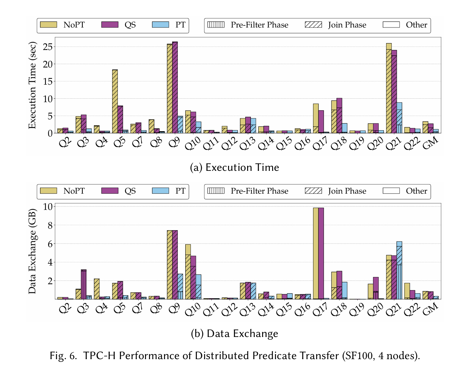
Fig. 6 has results for both end-to-end time, and the amount of data sent over the network. NoPT is the vanilla baseline, QS is prior work that tries to achieve a similar goal.

Source: https://dl.acm.org/doi/10.1145/3725259

Dangling Pointers

I’ve added the SlowRandomAccess tag to this one, Bloom filter insertion and probe operations require a small amount of compute, and then at least one random read/write. It would be amazing if there was another approximate membership testing algorithm that was more friendly to the memory hierarchy. In this paper, it seems like this could be a poor point for scalability, because at most steps there are multiple bloom filters at play, so the total working set for all bloom filters accessed by a single node in a single step is large.

In the shuffling case, bloom filter representations of subsets of R are sent across the network (nice for reducing networking bandwidth), but the actual contents of S must be sent. I believe this is because there is no efficient way to compute the intersection of two sets represented by two bloom filters.